VoxRay
VoxRay: Building a Real-Time Medical Volume Renderer with CUDA and ITK
I recently built VoxRay, a real-time DICOM volume renderer in C++/CUDA. The goal wasn’t to build a clinical tool, rather it was to get hands on experience with GPU accelerated data processing using CUDA, learn how medical imaging data is structured and loaded with ITK, and build a volume renderer from scratch without leaning on a high level engine. This post covers what I built, the interesting technical problems along the way, and what I learned.
What is volume rendering?
Most 3D rendering deals with surfaces built up of triangles, meshes, and normals. Volume rendering is different. Instead of surfaces, you have a 3D grid of density values, and the goal is to visualize that data in a meaningful way. Medical imaging is the classic use case: a CT scanner captures X-ray attenuation at thousands of points throughout the body, producing a 3D grid of Hounsfield unit (HU) values. Bone is dense and high HU, air is low HU, soft tissue falls somewhere in between.
The standard technique for rendering this data in real time is ray marching. For each pixel, cast a ray through the volume, sample the density at regular intervals along the ray, and accumulate color and opacity as you go. The result is something between an X-ray and 3D scan depending on how you tune the rendering parameters.
Loading DICOM data with ITK
Medical imaging data comes in DICOM format, a file format and network protocol standard used across virtually all clinical imaging hardware. A single CT scan is typically a directory of hundreds of .dcm files, one per slice.
I used ITK (Insight Toolkit) to handle the DICOM I/O. ITK is a large open source library used in medical image analysis research, and it handles the considerable complexity of DICOM parsing (series ordering, metadata extraction, pixel type handling) through a clean pipeline API:
					NamesGeneratorType::Pointer nameGenerator = NamesGeneratorType::New();
nameGenerator->SetDirectory(directory);

ReaderType::Pointer reader = ReaderType::New();
reader->SetImageIO(dicomIO);
reader->SetFileNames(nameGenerator->GetInputFileNames());
reader->Update();
After loading, I normallize the HU values to [0, 1] for the GPU pipeline using a two-pass approach: first find the min/max across all voxels, then normalize. For a 512x512x479 volume that’s 125 million voxels which is fast enough on the CPU for a one time preprocessing step, but a good candidate for GPU acceleration (more below).
The CUDA preprocessing pipeline
With the raw voxel data loaded, I run two CUDA preprocessing passes before the data ever touches the render pipeline.
Gaussian Smoothing
CT data has a fair amount of high frequency noise, which causes problems downstream when computing surface normals from density gradients. Noisy density means noisy gradients, which means noisy lighting. A Gaussian blur as a preprocessing step smooths this out.
I implemented this as a separable 3D convolution. Three 1D passes (X, Y, Z) rather than a full 3D kernel. A 3D Gaussian is mathematically separable, so this is equivalent but much cheaper: three passes of O(n·k) rather than one pass of O(n·k³) where k is the kernel radius.
Each pass is a CUDA kernel. The filter weights live in __constant__ memory, a 64KB read-only cache on the GPU that broadcasts a single value to all threads in a warp simultaneously, which is exactly the accesspattern for filter weights where every thread reads the same coefficients:
__constant__ float c_kernel[3] = { 0.25f, 0.5f, 0.25f };
I profiled the naive implementation with Nsight Compute and found the kernels running at 93% of peak memory bandwidth with only 30% compute throughput, classic memory bound behavior. The L1 cache hit rate was 38%, indicating threads were frequently going all the way to DRAM. The uncoalesced access pattern for the Y and Z passes (which stride across noncontiguous memory) accounts for the bulk of the remaining optimization opportunity, which shared memory tiling would address.
Gradient Computation for Surface Normals
After smoothing, I compute a gradient volume. For each voxel, the gradient of the density field approximated by central differences:
					float gx = sample(x+1, y, z) - sample(x-1, y, z);
float gy = sample(x, y+1, z) - sample(x, y-1, z);
float gz = sample(x, y, z+1) - sample(x, y, z-1);
float len = sqrtf(gx*gx + gy*gy + gz*gz);
float4 normal = (len > 1e-6f) ? make_float4(-gx/len, -gy/len, -gz/len, len) : make_float4(0.f, 0.f, 0.f, 0.f);
This is extremely parallel, every voxel is independent. The result is stored as float4 with the gradient magnitude in the w component, which I use later as a proxy for surface confidence when computing lighting. Both the density and normal volumes are uploaded to GPU as 3D textures for the render pipeline.
The Render Pipeline
Rendering happens in an OpenGL 4.3 compute shader. The GPU does the ray marching for every pixel in parallel. The pipeline is deferred style with separate albedo, depth, and normal passes written to image2D targets, then composited in a fragment shader.
Ray Marching
For each pixel, I compute a ray direction from the camera through the inverse view-projection matrix, tranform it into the volume’s local space to handle rotation without modifying the bounding box, then march through the volume accumulating color and opacity using front-to-back compositing.
I use jittered ray starts, offsetting each ray’s starting position by a random fraction of the step size, to break up the regular sampling pattern that causes banding artifacts. It’s a small change with a surprizingly large visual improvement.
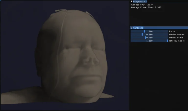
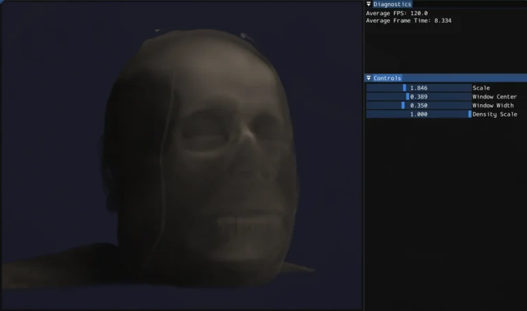
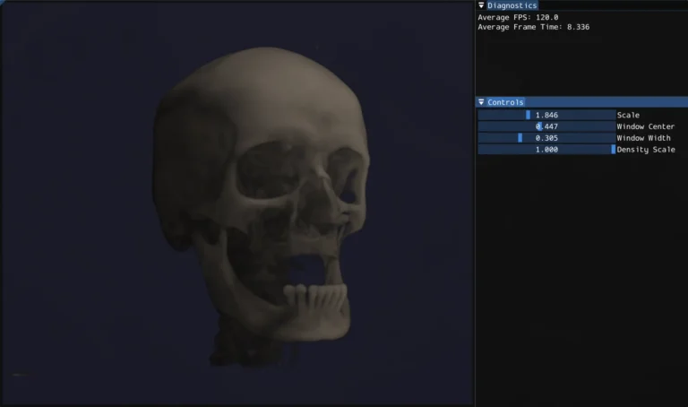
CT Windowing
One of the more medically interesting parts of the system is HU windowing. Rather than mapping the full density range to opacity, you specify a window center and width. Only values within that range are visible, and the mapping is linear within the window. This lets you isolate specific tissue types: narrow the window and center it on bone HU values and soft tissue becomes transparent, shift it lower and you see soft tissue structure instead.
Volumetric Lighting
Lighting in a volume renderer is more complex than surface rendering because there’s no single surface to light. Every sample along the ray contributes to the final color. I implemented single scattering: for each sample point that has non-zer density, cast a short shadow ray toward the light source and accumulate density along it. The Beer-Lambert law converts that accumulated density to a transmittance value. This gives self-shadowing throughout the volume. Dense regions cast shadows onto the material behind them, which is what makes the volume feel 3D rather than flat. The gradient normals from the CUDA preprocessing pass contribute a diffuse lighting term on top of this.
Physical Aspect Ratio
CT voxels aren’t always cubic. The in-plane resolution and slice thickness can differ. I extract voxel spacing from the DICOM metadata and pass it to the shader as a scale vector, so the bounding box matches the physical dimensions of the scan rather than stretching it into a unit cube.
What I learned
Cuda is approachable but optimization is deep. Writing correct parallel kernels is straightforward if you know C++ and have a mental model of GPU execution. The interesting part, and where real expertise lies, is performance optimization: understanding the memory hierarchy, designing access patterns for coalescing, using shared memory to reduce DRAM traffic, reading Nsight Compute output to find bottlenecks. Profiling the Gaussian blur and seeing 93% memory bandwidth utilization with only 30% compute throughput was a concrete lesson in what memory bound means in practice.
Mecial imaging has a lot of domain specific nuance. DICOM is more complex than it looks (series ordering, rescale intercepts, anisotropic voxel spacing, modality specific pixel representations). ITK abstracts most of this well, but understanding what it’s doing underneath matters for getting correct results.
Volume rendering quality comes from many small decisions. Jittered sampling, windowing, physical aspect ratio correction, gradient based normals, shadow ray length and step size are all minor in isolation, but together they’re the difference between something that looks like a blurry blob and something that looks like a head.
What’s next
The most interesting remaining work is proper transfer functions, mapping HU ranges to specific colors and opacities rather than the current linear mapping. That’s what makes clinical volume renderers look the way they do: bone rendered as opaque white, soft tissue as semi-transparent warm tones, air fully invisible. It would also open up the per tissue lighting possibilities that the normal volume is already set up to support.
On the CUDA side, the shared memory tiling optimization for the Gaussian blur passes is the natural next step. Loading volume tiles into __shared__ memory with halo borders to eliminate the repeated global memory reads and improve the L1 cache hit rate that Nsight identified.
Additional Resources
- Code Repository: GitHub Link